Think Correctly About ‘Liquidity’

Why Global Liquidity Matters

Fast-growing interest in understanding ‘liquidity’ has triggered a slew of misinformation on social media, which seem either to incorrectly challenge its importance or else emphasise the wrong measures. This short article tries to correct some of those errors.

Overview

Most investment analysis focuses on the inherent ‘value’ of individual securities, rather than the aggregate behaviour of investors. Liquidity analysis is concerned with macro-valuation shifts and tries to understand these movements from the behaviour and liability constraints of all investors, given the flows of funds into and out of financial markets. In short, it is an analysis of aggregate supply and demand across financial markets. The broad transmission process is illustrated below:

In this framework, generic asset prices (P) have two moving parts: (1) a pool of liquidity (L), and (2) the allocation of this liquidity to assets (P/L). Higher prices (P) can result either from more liquidity (L) and/ or a higher allocation to assets (P/L). An increase in liquidity can arise through Central Bank policy actions, as well as from lending decisions of private sector credit providers. Asset allocations depend on factors like investor sentiment, perceived inflation, tax rates and demographic trends.

The chart below shows the recent tight correlation between our measures of Global Liquidity – the flow of cash savings and credits flowing through World financial markets – and aggregate asset price movements, ie. World wealth (listed stocks and bonds, liquid assets, gold, precious metals, cryptocurrencies and residential real estate). We focus on Global Liquidity because, with unrestricted international capital movements, ultimately (outside of crises) all liquidity is fungible:

From experience, increases in stock market indexes, such as S&P500 and MSCI World Index, largely depend upon two factors – rising liquidity and falling inflation, because this incentivises higher allocations to stocks. See the chart below. This evidences how a fall in inflation from 6% to 4% leads to an increase in equity allocations (P/L) from o.35 to 0.55 times. This combination of rising liquidity and falling inflation largely explains our upbeat views towards stockmarkets in 2023.

For the record, the alternative model of projecting aggregate earnings (E) and a notional multiple (P/E) does not work well at the macro-level. Looking at aggregate P/Es would have led investors to miss the secular outperformance of Japanese equities through the 1980s and to have been near fully invested in European stocks over the last twenty years, thereby missing out of Wall Street’s stunning outperformance.

It turns out that the main driver of annual equity investment returns is changes in the aggregate P/E multiple, up to investment horizons of between 3-5 years. After that the earnings trend dominates. Drilling into the causes of P/E change, we can show that they are largely explained by the first two terms in square brackets (see below). These turn out to be the same asset allocation (P/L) and liquidity (L) factors that we described earlier. This shows how our approach is specifically designed to capture the key macro-valuation shifts that dominate markets:

Avoid Disinformation

Three false statements about liquidity are sometimes aired on social media sites. They remind us of the famous Groucho Marx quip about a restaurant’s awful food –  Groucho: “… and such small portions!”

(1)   US Fed Liquidity is simply US Banks’ Reserves and Reserves are not ‘money’ (a definitional question)

(2)  The Fed nor banks buy stocks directly so they should be unaffected (a question about transmission)

(3)  Statistically the relationship is weak (a factual question about results)

Fed Liquidity is not the same as Global Liquidity, but it is still an important aggregate. The statistical measure was originally devised at the US investment bank Salomon Brother Inc. and re-stated in our book Capital Wars (2020). This concept has gained popularity, especially in the past two years. Fed liquidity essentially consists of Fed credit (defined in the H4.1 release by the Fed) less notes and coins in circulation; less the reverse repo program (RRP); less the Treasury General Account (TGA) and plus any operating losses incurred by the Fed.

The chart below shows the recent co-movements between the level of Fed liquidity (US$ in billions) and the NASDAQ index. The relationship looks decent, but we should be wary of spurious correlation, question whether the relationship is causal and study whether it is sufficiently robust to work, say, in changes as well as levels?

Fed liquidity measures the net liquidity injections into US money markets. All money that is anywhere must, of course, be somewhere. Therefore, the arithmetic behind money market flows means that Fed liquidity should ultimately match the level of US banks’ reserves. See below:

Banks’ reserves are balances held at the Fed. They have credit/ liquidity balance sheet counterparts. Assume that the Fed purchases US Treasuries, provides direct lending and/ or repos securities. As a result, the private sector gets cash, and they may deposit the cash in US banks. The banks’ reserves rise. Collectively, the banking sector cannot get rid of these reserves. The most they can do is change the distribution and composition of the reserves. As much they try to purchase other assets or loans they cannot change the volume of reserves, which is ultimately determined by the Central Bank (and the US Treasury) through its credit activities. This means that banks’ balance sheets are likely to rise and fall with the supply of reserves by the Fed. The overall balance sheet capacity of the private sector is one way that we can measure ‘liquidity’.

Whether or not banks or Central Banks purchase stocks directly is plainly irrelevant, because there are second round effects from the expansion of Fed liquidity. These are portfolio rebalancing effects that, in our view, largely operate through the duration dimension. As liquidity increases as a proportion of the asset structure, average duration falls below liability duration targets. This triggers a reallocation of assets towards longer duration instruments. Correspondingly, these asset prices rise.

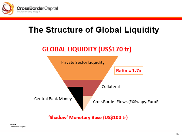
The schematic chart below shows the structure of Global Liquidity. This highlights how Fed liquidity (circa US$3 trillion) is just one part, albeit an important part, of the overall US$170 trillion pool of liquidity. Similarly, the same is true for World Central Bank liquidity. It is important but at some US$22 trillion in size, it is not the full picture.

We think of Global Liquidity creation comprising both a so-called shadow monetary base, consisting of Central Bank liquidity, offshore reservoirs of liquidity and collateral that can be used to support loans, and a muliplier. On top of this US$100 trillion base, private banks create liquidity. The multiplier between the shadow monetary base and the pool of Global Liquidity currently stands at 1.7 times.

Global Liquidity is large in size and evidently important, but does it drive asset markets as claimed? Robust statistical tests that try to counter the objections we raised earlier can be undertaken using a VAR (vector autoregression) model. The data set we use is weekly, starting from January 2010. The two tests we report below are: (1) impulse response of the MSCI World stock index to a positive Global Liquidity ‘shock’, and (2) a Granger causality test to better understand whether or not Global Liquidity one-way ‘causes’ movements in the MSCI World Index.

The chart below summaries the impulse responses. A positive liquidity shock appears to boost the MSCI index over an extended 12-week period (bottom axis):

The Granger causality results are given in the table below. These show that the probability that the MSCI does not ‘cause’ changes in Global Liquidity is 12.4%. This may appear ‘low’ but statistically it is unacceptable. At the same time, the probability that Global Liquidity does not cause changes in the MSCI Index is zero per cent. We conclude that the data likely reveal one-way statistical Granger causation between Global Liquidity and World stock markets.

Four Conclusions

·         Global Liquidity is the important monetary aggregate to monitor

·         Global Liquidity, in turn, comprises a multiplier times the World shadow Monetary Base

·         Transmission to asset prices occurs via portfolio rebalancings, These rebalancings are influenced by inflation, among other things

·         Global Liquidity statistically Granger causes future movements in asset prices